Examples
We consider several examples of the usage of ACBICI for the calibration of several models.
Example 0: using ACBICI for the first time
We describe in this example the simplest use of ACBICI. For that, we calibrate a well-known model and explore the features that ACBICI offers using as much as possible the pre-determined options that the library affords. All the files for this calibration can be found in the directory examples/example0. The four analyses can be run using the command make all.
The goal of example 0 is to obtain the value of gravity from a set of drop test measurements. A body is dropped from several heights and the time until its hits the floor is measure with a stopwatch. Following our description of the library, we say that the height \(h\) is the input variable, the time \(t\) until the body reaches the floor is the output, and gravity \(g\) is the only parameter whose value we would like to obtain. To do so, we use the classical expression
Since this simple formula ignores the aerodynamic forces, we expect it to be less accurate when the drop height \(h\) is large.
The first step to calibrate the model consists in gathering experimental data. In our case, we generate artificial data — as many as desired — using the function prepare.py. This function creates the file data/experiments.dat with one pair \((h_i,t_i)\) in every row, each of them corresponding to a fictitious experimental measurement.
The simplest possible calibration is obtained by running the Python program typeA.py. This program has two parts: first, the model to be calibrated is defined by initializing the parameter \(g\) and then providing the analytical expression of the model. Since we do not know much about gravity, we simply assume that its value is between \(7\) and \(12\), and use a uniform probability distribution as its prior. This is the corresponding code:
class myModel(ACBICImodel):

    def __init__(self):
        self.xdim = 1
        self.addParameter(label=r'$g$', prior=Uniform(a=7.0, b=12.0))


    def symbolicModel(self, x, p):
        x = to_column_vector(x)
        p = to_column_vector(p)
        r = np.sqrt(2.0*x[:,0]/p[:,0])
        r = to_column_vector(r)
        return r
In the second part, the analysis creates a classicalCalibrator object by combining the experimental data and the symbolic model. This is the simplest analysis possible, and it will run classical a Bayesian inference algorithm. Last, simply by calling the calibrate method, ACBICI would take care of all the process
theModel = myModel()
experiments = np.loadtxt("data/experiments.dat")

theCalibrator = classicalCalibrator(theModel)
theCalibrator.storeExperimentalData(experiments)
theCalibrator.calibrate()
theCalibrator.printReport()
theCalibrator.plot()
This program creates a directory with a unique random name. Inside it, the user may find a report with the information obtained from the calibration, as well as figures for the calibrated model, the probability distribution of the parameter \(g\) and the experimental error, and more.
In order to calibrate a model using Bayesian methods, the symbolic model needs to be evaluated thousands of times. In the example under consideration this entails very little cost since the model consists, essentially, of a single line of Python code. In other cases, however, the model is so expensive that this approach is not practical. In the second type of analysis considered, the model is replaced by a surrogate which, in theory, is much more efficient than the actual model. In the drop-test example, this is not the case but, nevertheless, we provide the code that shows the necessary steps to do so whenever it becomes necessary.
The analysis of this “expensive” model can be found in typeB.py. Here, the calibration consists, as before, of two parts: the definition of the model itself, and the calibration. Since the first part is identical to the one in typeA.py we just show the second part.
theModel = myModel()
experiments = np.loadtxt("data/experiments.dat")
theCalibrator = expensiveCalibrator(theModel)
theCalibrator.storeExperimentalData(experiments)
theCalibrator.calibrate()
theCalibrator.printReport()
theCalibrator.plot()
As in the standard calibration, the output of this second calibration will be written to files inside a directory with a unique random name. There, one can find the analysis report as well as figures with relevant information.
Often, it turns out that the model we want to calibrate does not fit well the experimental data. Maybe the model is too simplistic or somehow we have considered a wrong functional form for it. Whatever the reasons maybe, we say that the model has some inherent discrepancy with the data that can not be eliminated irrespective of the parameter choice. ACBICI allows to quantify this functional discrepancy by using a discrepancyCalibrator. Employing the latter, in addition to estimating the most likely probability distribution of the model parameters, a model-free discrepancy function is also estimated. In the case of the drop-tests, the discrepancy function should reveal that the classical formula \(t=\sqrt{2 h/g}\) ignores air resistance. Hence, large modeling error should be expected when dropping objects from large heights. The code that runs this analysis, taken from the file typeC.py, is
theModel = myModel()
experiments = np.loadtxt("data/experiments.dat")
theCalibrator = discrepancyCalibrator(theModel, name="typeC")
theCalibrator.storeExperimentalData(experiments)
theCalibrator.calibrate(nsteps=20000)
theCalibrator.printReport()
theCalibrator.plot()
Here, the results of the analysis are written inside a directory called typeC, since we have provided a special argument to the calibrator constructor.
Finally, it might be case that the model whose parameters and discrepancy we would like to estimate is so expensive that a surrogate model needs to be used, just like in the type B analysis. In these situations, a KOHCalibrator will perform the desired tasks. The code that needs to be used to run such analysis is in file typeD.py and contains the block:
theModel = myModel()
experiments = np.loadtxt("data/experiments.dat")
theCalibrator = KOHCalibrator(theModel, name="typeD")
theCalibrator.storeExperimentalData(experiments)
theCalibrator.calibrate()
theCalibrator.printReport()
theCalibrator.plot()
Example 1: a one parameter model
This simple example is provided in file examples/multiple01.py and implements in a compact way all the calibration strategies allows in ACBICI. The experimental data required for the calibration is artificially manufactured so that each time that the calibration is run a new set of “experimental” data is employed. This (fake) experimental data is stored in the file experiments.dat. For the expensive calibrators, synthetic data must be generated by sampling the input and parameter spaces. These data are stored – and loaded later – in the file synthetic.dat.
The model is, as required, defined by sub-classing the abstract class ACBICImodel and providing the initialization and evaluation functions:
class myModel(ACBICImodel):

    def __init__(self):
        self.xdim = 1
        self.addParameter(label=r'$\theta$', prior=Uniform(a=1.0, b=2.0))


    def symbolicModel(self, x, p):
        r = np.sin(x[:,0]*p[:,0]) + x[:,0]*0.1
        return r
The analysis Python file is shown next. After creating the model and generating the (fake) experimental data and the synthetic samples, ten different calibrations are performed.
theModel = myModel()
cookupExperimentalData(20, "data/experiments.dat")
experiments = np.loadtxt("data/experiments.dat")
cookupSyntheticData(theModel, 20, "data/experiments.dat")
sd = np.loadtxt("data/experiments.dat")

print("*** Type A calibration + known experimental error")
theCalibrator = classicalCalibrator(theModel, name="calA")
theCalibrator.setExperimentalSTDValue(0.1)
theCalibrator.storeExperimentalData(experiments)
theCalibrator.calibrate()
theCalibrator.printReport()
theCalibrator.plot(onscreen=False)

print("*** Type A calibration + unknown experimental error")
theCalibrator = classicalCalibrator(theModel)
theCalibrator.setExperimentalSTDPrior(Gamma(alpha=2,beta=2))
theCalibrator.storeExperimentalData(experiments)
theCalibrator.calibrate(nsteps=10000, burn=0.2, thin=1, nwalkers=16)
theCalibrator.printReport()
theCalibrator.plot(dumpfiles=False,onscreen=False)

print("*** Type B calibration + known experimental error")
theCalibrator = expensiveCalibrator(theModel, name="calB")
theCalibrator.setExperimentalSTDValue(0.1)
theCalibrator.storeExperimentalData(experiments)
theCalibrator.calibrate(nsteps=20000, burn=0.1)
theCalibrator.printReport()
theCalibrator.plot(trace=False,onscreen=False)

print("*** Type B calibration + unknown experimental error + auto synthetic")
theCalibrator = expensiveCalibrator(theModel, name="calBE")
theCalibrator.setExperimentalSTDPrior(Gamma(alpha=2,beta=2))
theCalibrator.storeExperimentalData(experiments)
theCalibrator.calibrate(nsteps=10000)
theCalibrator.printReport()
theCalibrator.plot(onscreen=False)

print("*** Type B calibration + known experimental error + external synthetic")
theCalibrator = expensiveCalibrator(theModel)
theCalibrator.setExperimentalSTDValue(0.5)
theCalibrator.storeExperimentalData(experiments)
theCalibrator.storeSyntheticData(sd)
theCalibrator.calibrate(nsteps=20000, burn=0.1)
theCalibrator.printReport()
theCalibrator.plot(onscreen=False)

print("*** Type C calibration + known experimental error")
theCalibratorC = discrepancyCalibrator(theModel, name="calC")
theCalibratorC.setExperimentalSTDValue(0.1)
theCalibratorC.storeExperimentalData(experiments)
theCalibratorC.calibrate(thin=1, nwalkers=16, nsteps=10000)
theCalibratorC.printReport()
theCalibratorC.plot(trace=False,onscreen=False)

print("*** Type C calibration + unknown experimental error")
theCalibrator = discrepancyCalibrator(theModel, name="calCE")
theCalibrator.setExperimentalSTDPrior(Gamma(alpha=2,beta=2))
theCalibrator.storeExperimentalData(experiments)
theCalibrator.calibrate()
theCalibrator.printReport()
theCalibrator.plot(onscreen=False)

print("*** Type D calibration + known experimental error + auto synthetic")
theCalibrator = KOHCalibrator(theModel, name="calD")
theCalibrator.setExperimentalSTDValue(0.1)
theCalibrator.storeExperimentalData(experiments)
theCalibrator.calibrate(nsteps=20000)
theCalibrator.printReport()
theCalibrator.plot(onscreen=False)

print("*** Type D calibration + known experimental error + external synthetic")
theCalibrator = KOHCalibrator(theModel)
theCalibrator.setExperimentalSTDValue(0.5)
theCalibrator.storeExperimentalData(experiments)
theCalibrator.storeSyntheticData(sd)
theCalibrator.calibrate(nsteps=20000)
theCalibrator.printReport()
theCalibrator.plot(trace=False,onscreen=False)

print("*** Type D calibration + unknown experimental error + auto synthetic")
theCalibrator = KOHCalibrator(theModel, name="calDe")
theCalibrator.setExperimentalSTDPrior(Gamma(alpha=2,beta=2))
theCalibrator.storeExperimentalData(experiments)
theCalibrator.calibrate(nsteps=25000)
theCalibrator.printReport()
theCalibrator.plot(trace=True, corner=True, dumpfiles=True, onscreen=False)
Example 2: a two-parameter model
This second example extends the previous one by considering a model that has two parameters to be calibrated. The model itself is defined, as explained, by deriving a class from the abstract class ACBICImodel, and providing the functions __init__ and symbolicModel. Note that the two parameters of the problem are \(\theta\) and \(\zeta\).
class myModel(ACBICImodel):

   def __init__(self):
       self.xdim = 1
       self.addParameter(label=r'$\theta$', prior=Uniform(a=1.0, b=1.5))
       self.addParameter(label=r'$\zeta$', prior=Normal(mu=0.0, sigma=1.0))

   def symbolicModel(self, x, p):
       xc = x[:,0]
       theta = p[:,0]
       zeta = p[:,1]
       r = np.sin(theta*xc) + zeta*xc
       return r
Running the calibration process for this third model follows the identical process employed in example 1. In fact, this structure can be used to calibrate an arbitrary model by selecting one of the ten different calibration examples shown below.
theModel = myModel()
cookupExperimentalData(30, "data/experiments.dat")
experiments = np.loadtxt("data/experiments.dat")
cookupSyntheticData(theModel, 20, "data/experiments.dat")
sd = np.loadtxt("data/experiments.dat")

print("*** Type A calibration + known experimental error")
calibratorA = classicalCalibrator(theModel, name="calA")
calibratorA.setExperimentalSTDValue(0.05)
calibratorA.storeExperimentalData(experiments)
calibratorA.calibrate()
calibratorA.printReport()
calibratorA.plot(onscreen=True)

print("*** Type A calibration + unknown experimental error")
calibratorAexp = classicalCalibrator(theModel, name="calAE")
calibratorAexp.setExperimentalSTDPrior(Gamma(alpha=2,beta=2))
calibratorAexp.storeExperimentalData(experiments)
calibratorAexp.calibrate(nsteps=15000, burn=0.2, thin=1, nwalkers=16)
calibratorAexp.printReport()
calibratorAexp.plot()

print("*** Type B calibration + known experimental error")
calibratorB = expensiveCalibrator(theModel, name="calB")
calibratorB.setExperimentalSTDValue(0.05)
calibratorB.storeExperimentalData(experiments)
calibratorB.calibrate(nsteps=15000, burn=0.1)
calibratorB.printReport()
calibratorB.plot()

print("*** Type B calibration + unknown experimental error")
calibratorBexp = expensiveCalibrator(theModel, name="calBE")
calibratorBexp.setExperimentalSTDPrior(Gamma(alpha=2,beta=2))
calibratorBexp.storeExperimentalData(experiments)
calibratorBexp.calibrate(nsteps=10000)
calibratorBexp.printReport()
calibratorBexp.plot(onscreen=False)

print("*** Type C calibration + known experimental error")
calibratorC = discrepancyCalibrator(theModel, name="calC")
calibratorC.setExperimentalSTDValue(0.05)
calibratorC.storeExperimentalData(experiments)
calibratorC.calibrate(thin=1, nwalkers=16)
calibratorC.printReport()
calibratorC.plot()

print("*** Type C calibration + unknown experimental error")
calibratorCexp = discrepancyCalibrator(theModel, name="calCE")
calibratorCexp.setExperimentalSTDPrior(Gamma(alpha=2,beta=2))
calibratorCexp.storeExperimentalData(experiments)
calibratorCexp.calibrate()
calibratorCexp.printReport()
calibratorCexp.plot()

print("*** Type D calibration + known experimental error + auto synthetic")
theCalibrator = KOHCalibrator(theModel, name="calD")
theCalibrator.setExperimentalSTDValue(0.05)
theCalibrator.storeExperimentalData(experiments)
theCalibrator.replaceHyperparameterPrior(label=r'$\beta_x', prior=Gamma(alpha=2.0, beta=.5))
theCalibrator.replaceHyperparameterPrior(label=r'$\beta_t', prior=Gamma(alpha=2.0, beta=.5))
theCalibrator.calibrate(nsteps=30000, nsynthetic=50)
theCalibrator.printReport()
theCalibrator.plot(onscreen=True)

print("*** Type D calibration + known experimental error + external synthetic")
theCalibrator = KOHCalibrator(theModel)
theCalibrator.setExperimentalSTDValue(0.05)
theCalibrator.storeExperimentalData(experiments)
theCalibrator.storeSyntheticData(sd)
theCalibrator.calibrate(nsteps=40000, nsynthetic=40)
theCalibrator.printReport()
theCalibrator.plot(trace=False, onscreen=False)

print("*** Type D calibration + unknown experimental error + auto synthetic")
theCalibrator = KOHCalibrator(theModel, name="calDe")
theCalibrator.setExperimentalSTDPrior(Gamma(alpha=2,beta=2))
theCalibrator.storeExperimentalData(experiments)
theCalibrator.calibrate(nsteps=25000)
theCalibrator.printReport()
theCalibrator.plot(trace=True, corner=True, dumpfiles=True, onscreen=False)
Example 3: Cobb-Douglas Production model
This example uses the Cobb-Douglas production model, a well-known function in economics. It relates total output to the levels of labor and capital input, scaled by a productivity factor.
The model assumes that the total output \(Y\) is a function of:
\(L\) — labor used in production
\(K\) — capital used in production
\(T\) — total factor productivity
The model takes the following mathematical form:
Input variables: \(T\), \(L\), \(K\) Model parameters: \(\alpha\), \(\gamma\)
The model itself is defined, as explained, by deriving a class from the abstract class ACBICImodel, and providing the functions __init__ and symbolicModel.
This setup defines a 3-dimensional input space with 2 model parameters to be calibrated.
Input Scaling
Note that the original input dimensions had significantly different scales. Among the input variables, \(T\) (total factor productivity) is assumed to take values in the normalized range \([0, 1]\). The other inputs, \(L\) (labor) and \(K\) (capital), originally have different physical scales and are nondimensionalized by dividing by characteristic reference values:
\(L_0 = 50\)
\(K_0 = 200\)
This yields the scaled inputs:
Thus, the final nondimensionalized input vector becomes:
This normalization ensures that each input contributes comparably during calibration, which is important for numerical stability and interpretability.
class myModel(ACBICImodel):

def __init__(self):
     self.xdim = 3
     self.addParameter(label=r'$\alpha$', prior=Uniform(a=0.3, b=1.6))
     self.addParameter(label=r'$\gamma$', prior=Normal(mu=0.35, sigma=0.1))

def symbolicModel(self, x, p):
     # Inputs should be of shape (nexp, xdim) and (nexp, pdim)
     # The output must be of shape (nexp, ydim)
     T = x[:, 0]
     L = x[:, 1]
     K = x[:, 2]

     alpha = p[:, 0]
     gamma = p[:, 1]

     r = T * L**alpha * K**gamma
     return r.reshape(-1, 1)
The calibration process for this fourth model is identical to the procedure used in Examples 1 and 2. This modular structure can be applied to calibrate arbitrary models by selecting from any of the nine calibration examples provided below.
print("*** Type A calibration + known experimental error")
calibratorA = classicalCalibrator(theModel, name="calA")
calibratorA.setExperimentalSTDValue(0.05)
calibratorA.storeExperimentalData(experiments)
calibratorA.calibrate()
calibratorA.printReport()
calibratorA.plot(onscreen=False, compare=True)

print("*** Type A calibration + unknown experimental error")
calibratorAexp = classicalCalibrator(theModel, name="calAE")
calibratorAexp.storeExperimentalData(experiments)
calibratorAexp.calibrate(nsteps=15000, burn=0.2, thin=1, nwalkers=16)
calibratorAexp.printReport()
calibratorAexp.plot(compare=False, onscreen=False)

print("*** Type C calibration + known experimental error")
calibratorC = discrepancyCalibrator(theModel, name="calC", kernel="matern32")
calibratorC.setExperimentalSTDValue(0.05)
calibratorC.storeExperimentalData(experiments)
calibratorC.calibrate(thin=1, nwalkers=16, nsteps=15000)
calibratorC.printReport()
calibratorC.plot()

print("*** Type C calibration + unknown experimental error")
calibratorCexp = discrepancyCalibrator(theModel, name="calCE")
calibratorCexp.setExperimentalSTDPrior(HalfCauchy(mu=0.05, sigma=0.1))
calibratorCexp.storeExperimentalData(experiments)
calibratorCexp.calibrate(nsteps=20000)
calibratorCexp.printReport()
calibratorCexp.plot()

print("*** Type B calibration + known experimental error")
calibratorB = expensiveCalibrator(theModel, name="calB")
calibratorB.setExperimentalSTDValue(0.05)
calibratorB.storeExperimentalData(experiments)
calibratorB.calibrate(nsteps=15000, burn=0.1)
calibratorB.printReport()
calibratorB.plot(compare=True, onscreen=False)

print("*** Type B calibration + unknown experimental error")
calibratorBexp = expensiveCalibrator(theModel, name="calBE")
calibratorBexp.setExperimentalSTDPrior(Gamma(alpha=2,beta=2))
calibratorBexp.storeExperimentalData(experiments)
calibratorBexp.calibrate(nsteps=15000)
calibratorBexp.printReport()
calibratorBexp.plot(onscreen=False)

print("*** Type D calibration + known experimental error + auto synthetic")
theCalibrator = KOHCalibrator(theModel, name="calD")
theCalibrator.setExperimentalSTDValue(0.05)
theCalibrator.storeExperimentalData(experiments)
theCalibrator.replaceHyperparameterPrior(label=r'$\beta_x$', prior=Gamma(alpha=5., beta=2.))
theCalibrator.calibrate(nsteps=30000, nsynthetic=50)
theCalibrator.printReport()
theCalibrator.plot()

print("*** Type D calibration + known experimental error + external synthetic")
theCalibrator = KOHCalibrator(theModel)
theCalibrator.setExperimentalSTDValue(0.05)
theCalibrator.storeExperimentalData(experiments)
#theCalibrator.replaceHyperparameterPrior(label=r'$\lambda_d$', prior=Gamma(alpha=2., beta=2.))
theCalibrator.storeSyntheticData(sd)
theCalibrator.calibrate(nsteps=30000)
theCalibrator.printReport()
theCalibrator.plot(trace=False, onscreen=False)

print("*** Type D calibration + unknown experimental error + auto synthetic")
theCalibrator = KOHCalibrator(theModel, name="calDE")
theCalibrator.setExperimentalSTDPrior(HalfCauchy(mu=0.1, sigma=0.1))
theCalibrator.storeExperimentalData(experiments)
theCalibrator.calibrate(nsteps=30000)
theCalibrator.printReport()
theCalibrator.plot(trace=True, corner=True, dumpfiles=True, onscreen=False)
Example 4: Traction test
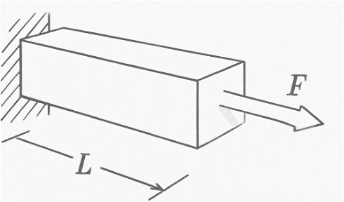
This example considers a traction test with either the first (example4_1stobjective), the second (example4_2ndobjective) or both outputs/tasks (example4_biobjective). The problem involves the following quantities:
where:
\(L\) is the initial length of the specimen.
\(A\) is the initial cross-sectional area of the specimen.
\(F\) is the applied traction force.
\(E\) is the Young’s modulus (elastic modulus) of the material.
\(\nu\) is the Poisson’s ratio of the material.
\(y_1\) is the resulting length under the applied force.
\(y_2\) is the resulting cross-sectional area under the applied force.
This formulation assumes the material is elastic and isotropic, following linear elasticity theory.
Nondimensionalization
When working with ACBICI, it is important to nondimensionalize your equations. This becomes certainly unavoidable when aiming for multivariate calibration. Here, we demonstrate this for the traction test:
The following reference (characteristic) constants are used:
Reference Young’s modulus: \(E_0 = 250\,\text{MPa}\)
Reference width: \(b = 1\,\text{mm}\)
Reference height: \(h = 1\,\text{mm}\)
Reference area: \(A_0 = b \times h = 1\,\text{mm}^2\)
Reference length: \(L_0 = 10\,\text{mm}\)
Reference force: \(F_0 = E_0 \times A_0 = 250\,\text{N}\)
All quantities are nondimensionalized as follows:
The nondimensional outputs are:
For the specific geometry in the code (\(L = L_0\), \(A = A_0\)), \(L_{\mathrm{hat}} = 1\) and \(A_{\mathrm{hat}} = 1\).
Model Definition
This ensures all outputs are unitless and directly comparable. Then we can define the model as for the previous examples, where for example4_biobjective, we have to set the output dimension to 2:
class myModel_nondim(ACBICImodel):

  def __init__(self):
      self.xdim = 1
      self.ydim = 2
      E0 = 250.
      self.addParameter(label=r'$E$', prior=Uniform(a=200.0/E0, b=400.0/E0))
      self.addParameter(label=r'$\nu$', prior=Uniform(a=0.0, b=0.5))

  def symbolicModel(self, x, p):
      # Inputs should be of shape nexp x xdim and nexp x pdim not (nexp,)
      # and return something of shape (nexp,ydim) not (nexp,)
      # Ensure x is a 2D array (n_samples, 1) for proper indexing
      x = np.atleast_2d(x)  # Convert x to a 2D array if it's not already
      p = np.atleast_2d(p)  # Convert p to a 2D array if it's not already

      L = 10.
      b = 1
      h = 1
      A = b * h  # rectangular beam
      A0 = A
      L0 = 10
      A_hat = A/A0
      L_hat = L/L0
      r1 = L_hat * (1 + x[:, 0] / (A * p[:,0]))  #length
      r2 = A_hat * (1 - x[:, 0] * p[:,1] / (A * p[:,0]))**2  #new area

      r = np.column_stack([r1,r2])
      return r
Calibration Process
The calibration process works as for the other examples. You can run different calibration types by executing one or all of the eight examples provided below.
print("*** Type A calibration + known experimental error")
theCalibrator = classicalCalibrator(theModel, name="calA")
theCalibrator.setExperimentalSTDValue(0.02)
theCalibrator.storeExperimentalData(experiments)
theCalibrator.calibrate(thin=1, nwalkers=16, nsteps=10000)
theCalibrator.printReport()
theCalibrator.plot(dumpfiles=True, onscreen=False)
print("########################################################")

print("*** Type A calibration + unknown experimental error")
theCalibrator = classicalCalibrator(theModel, name="calAE")
theCalibrator.storeExperimentalData(experiments)
theCalibrator.calibrate(nsteps=15000, burn=0.2, thin=1, nwalkers=16)
theCalibrator.printReport()
theCalibrator.plot(dumpfiles=True, onscreen=False)

print("*** Type C calibration + known experimental error")
theCalibrator = discrepancyCalibrator(theModel, name="calC")
theCalibrator.setExperimentalSTDValue(0.02)
theCalibrator.storeExperimentalData(experiments)
theCalibrator.calibrate(thin=1, nwalkers=16, nsteps=20000)
theCalibrator.printReport()
theCalibrator.plot(dumpfiles=True, onscreen=False)

print("*** Type C calibration + unknown experimental error")
theCalibrator = discrepancyCalibrator(theModel, name="calCE")
theCalibrator.setExperimentalSTDPrior(HalfCauchy(mu=0.0, sigma=0.1))
theCalibrator.storeExperimentalData(experiments)
theCalibrator.calibrate(nsteps=20000)
theCalibrator.printReport()
theCalibrator.plot(onscreen=False)

print("*** Type B calibration + known experimental error")
theCalibrator = expensiveCalibrator(theModel, name="calB")
theCalibrator.setExperimentalSTDValue(0.02)
theCalibrator.storeExperimentalData(experiments)
theCalibrator.storeSyntheticData(sd)
theCalibrator.calibrate(thin=1, burn=0.2, nwalkers=16, nsteps=20000)
theCalibrator.printReport()
theCalibrator.plot(dumpfiles=True, onscreen=False)

print("*** Type B calibration + unknown experimental error")
theCalibrator = expensiveCalibrator(theModel, name="calBE")
theCalibrator.storeExperimentalData(experiments)
theCalibrator.storeSyntheticData(sd)
theCalibrator.calibrate(thin=1, burn=0.2, nwalkers=16, nsteps=20000)
theCalibrator.printReport()
theCalibrator.plot(dumpfiles=True, onscreen=False)

print("*** Type D calibration + known experimental error + external synthetic")
theCalibrator = KOHCalibrator(theModel, name="calD")
theCalibrator.setExperimentalSTDValue(0.02)
theCalibrator.storeExperimentalData(experiments)
theCalibrator.storeSyntheticData(sd)
theCalibrator.calibrate(thin=1, burn=0.2, nwalkers=16, nsteps=20000)
theCalibrator.printReport()
theCalibrator.plot(onscreen=False, dumpfiles=True)

print("*** Type D calibration + unknown experimental error + external synthetic")
theCalibrator = KOHCalibrator(theModel, name="calDE")
theCalibrator.setExperimentalSTDPrior(HalfCauchy(mu=0.0, sigma=0.1))
theCalibrator.storeExperimentalData(experiments)
theCalibrator.storeSyntheticData(sd)
theCalibrator.calibrate(thin=1, burn=0.2, nwalkers=16, nsteps=20000)
theCalibrator.printReport()
theCalibrator.plot(dumpfiles=True, onscreen=False)
Sobol Sensitivity Analysis
For this example, a Sobol Sensitivity Analysis can be performed by running the following routine.
def analyze_sensitivity(time):
    # time as 2d vector
    problem = {
        'num_vars': 2,
        'names': ['p0', 'p1'],
        'bounds': [[200.0/250., 400.0/250.],  # Range for p0
                   [0.0, 0.50]]    # Range for p1
    }

    # Generate samples using Saltelli sampling
    param_values = sobol.sample(problem, 1024)

    # Run the model for each parameter sample
    Y = np.array(
        [theModel.symbolicModel(time, p.reshape(1, -1)).sum()
         for p in param_values])

    # Perform Sobol sensitivity analysis
    Si = sobol_analyze.analyze(problem, Y)

    print("First-order Sobol indices:", Si['S1'])
    print("Total Sobol indices:", Si['ST'])
Sobol sensitivity analysis is a variance-based global sensitivity method that quantifies how the uncertainty in each model parameter contributes to the variance in the output—both individually and via interactions.
In this example, we apply Sobol analysis to the nondimensional parameters:
\(E_\mathrm{hat}\) (nondimensional Young’s modulus)
\(\nu_\mathrm{hat}\) (nondimensional Poisson’s ratio)
Parameter ranges are:
For each output of interest (such as \(y_1\) and \(y_2\)), the analysis computes:
First-order Sobol indices (\(S_1\)): Proportion of output variance attributed to each parameter alone.
Total-effect Sobol indices (\(S_T\)): Proportion of output variance attributed to each parameter, including all its interactions.
Mathematically, the output variance is decomposed as:
where \(V_i\) is the variance due to parameter \(i\) alone, and \(V_{ij}\) is due to the interaction of parameters \(i\) and \(j\).
The first-order index for parameter \(i\) is
and the total-effect index is
Interpretation:
If \(S_i\) is large, parameter \(i\) alone strongly determines the output.
If \(S_{T_i} - S_i\) is large, the parameter is important mainly through interactions.
If both indices are small, the parameter is not influential.
This approach allows us to identify which nondimensionalized parameters most affect the model predictions, guiding calibration and experimental design.
Implementation note: Saltelli sampling is used to efficiently generate parameter sets and compute the model output for each, then estimate Sobol indices for each output.